Review on Difference Between 2 Means Z Distribution
Two-sample Inference for the Difference Between Groups with Python
College Statistics with Python
Introduction
In a series of weekly articles, I volition cover some important statistics topics with a twist.
The goal is to use Python to assist us get intuition on complex concepts, empirically exam theoretical proofs, or build algorithms from scratch. In this series, you will find articles roofing topics such as random variables, sampling distributions, confidence intervals, significance tests, and more.
At the finish of each commodity, you can find exercises to examination your knowledge. The solutions volition be shared in the article of the following calendar week.
Articles published so far:
- Bernoulli and Binomial Random Variables with Python
- From Binomial to Geometric and Poisson Random Variables with Python
- Sampling Distribution of a Sample Proportion with Python
- Confidence Intervals with Python
- Significance Tests with Python
- Two-sample Inference for the Deviation Between Groups with Python
- Inference for Categorical Data
- Advanced Regression
- Assay of Variance — ANOVA
As usual, the code is bachelor on my GitHub.
Comparison Population Proportions
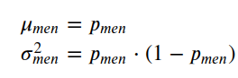
Imagine that i of the candidates for Porto's city was interested in comparison the proportion of men and women that volition vote for him. During that weekend, a new poll comes out with the following information: from a sample of m men, 62% answered that volition vote for him, and from a sample of 1000 women, 57% answered that will vote for him. These are, in reality, ii Bernoulli distributions which nosotros can ascertain by the parameters:
from scipy.stats import bernoulli, norm
import numpy as np
import seaborn as sns
import math
import matplotlib.pyplot as plt
from graphviz import Digraph # Theoretical parameters for men
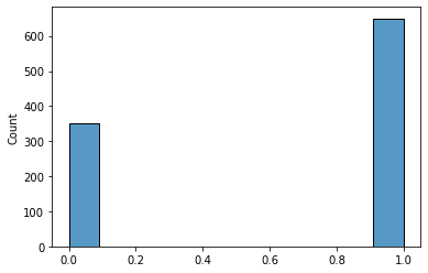
p1 = 0.65
n1=1000
n = n1μ_1 = p1
var_1 = p1*(1-p1)dist_men = np.concatenate((np.ones(int(p1*n)), np.zeros(int(n-(p1*n)))))
sns.histplot(dist_men);
# Theoretical parameters for women
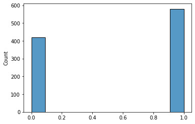
p2 = 0.58
n2 = northμ_2 = p2
var_2 = p2*(i-p2)
dist_women = np.concatenate((np.ones(int(p2*n)), np.zeros(int(n-(p2*n)))))
sns.histplot(dist_women);
We want to figure out if there is a meaningful difference in the manner men and women vote for the candidate. In reality, we want to come up up with a 95% confidence interval for that departure.
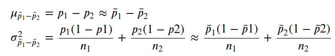
Considering the sample size is big enough, we can assume that a normal distribution can judge the sampling distributions of the sample proportions. In previous manufactures, we already saw some of the properties of these distributions:
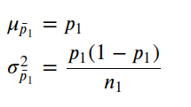
Notice that they took 1000 samples from the original distribution to create the poll so calculated the mean from that sample. This procedure is equivalent to taking a sample from the sampling distribution of sample proportions.
          # Sampling distribution of sample proportion for menmu = p1
variance = p1*(i-p1)/n
sigma = math.sqrt(variance)
x = np.linspace(mu - 3*sigma, mu + three*sigma, 100)
sns.lineplot(x = x, y = norm.pdf(x, mu, sigma));
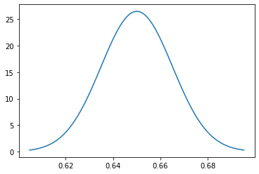
Sampling distribution of sample proportion for men. # Sampling distribution of sample proportion for womenmu = p2
variance = p2*(i-p2)/n
sigma = math.sqrt(variance)
x = np.linspace(mu - 3*sigma, mu + 3*sigma, 100)
sns.lineplot(x = 10, y = norm.pdf(x, mu, sigma));
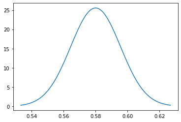
Sampling distribution of sample proportion for women. In fact, we are non interested in the individual distributions for men and women. Our interest is in their differences, so let'due south create the sampling distribution of

For that, we need to define its parameters:
          # Sampling distribution of sample proportion for the difference between men and womenmu = p1-p2
variance = p1*(1-p1)/northward + p2*(one-p2)/n
sigma = math.sqrt(variance)
x = np.linspace(mu - three*sigma, mu + three*sigma, 100)
sns.lineplot(ten = 10, y = norm.pdf(10, mu, sigma));
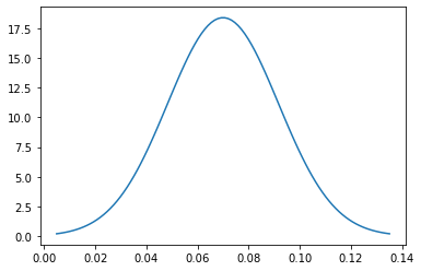
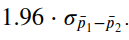
Figure half dozen: Sampling distribution of sample proportion for the difference between men and women. The confidence interval that we want to summate states that there is a 95% adventure that p1-p2 is within
# Computing the number of standard deviations required for a 95% intervalnorm.ppf(0.975)
i.959963984540054
Allow's calculate our interval.
np.sqrt(variance) * norm.ppf(0.975) 0.042540701104107376
Now we know that there is a 95% chance that the true departure of the proportions is within 0.04254 of the bodily difference of the sample proportions.
print(f'The 95% CI is: [{np.circular(p1-p2 - np.sqrt(variance) * norm.ppf(0.975), 3)},{np.round(p1-p2 + np.sqrt(variance) * norm.ppf(0.975), 3)}]') The 95% CI is: [0.027,0.113]
The candidate can conclude that there is a 95% take a chance that men are more probable to vote for him than women. Observe that the value 0 (no difference) is not independent in the interval.
Hypothesis test comparison population proportions
We tin can exist fifty-fifty more direct in our arroyo. Nosotros can define a hypothesis test to evaluate if, in fact, that is a difference.
We start by defining our null hypothesis, which represents the no divergence scenario. Conversely, our alternative hypothesis states that there is a difference.
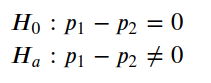
Thus, we want to summate
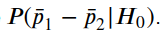
If this probability is less than the significance level defined for the trouble, we volition refuse our zilch hypothesis and accept a deviation betwixt how men and women vote for the candidate. In other words, assuming that the true proportions are equal, we want to know the probability of getting something every bit farthermost as the value of the difference of the sampling proportions. We tin define our z-score equally,
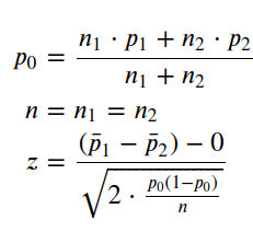
          p0 = (n1*p1+n2*p2)/(n1+n2)
z = ((p1 - p2) - 0) /(np.sqrt(2*(p0*(1-p0)/n)))
z          3.2167337783899304
We can now compare our z-statistic with the critical value for a significance level of v%.
          z_critical = norm.ppf(0.975)
z_critical          1.959963984540054          z > z_critical          True
Our z-statistic is greater than the critical value. In other words, there is a 5% chance of sampling a z-statistic greater than the disquisitional value assuming our aught hypothesis. In this scenario, we reject H_0, which means that we take a difference betwixt men and women voting for the candidate.
Statistical Significance of Experiment
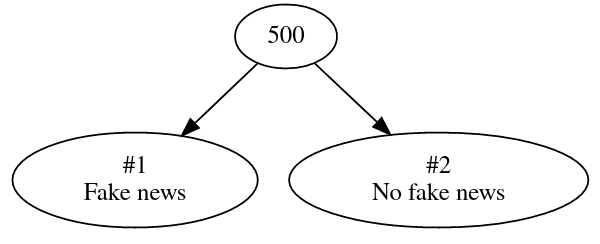
In an experiment aimed at studying the outcome of faux news on appointment, a group of 500 people was randomly assigned to two different groups. Subsequently randomization, each person received a smartphone with just a social media app that they could use to follow the news and updates from their friends.
The showtime group received fake news at least 2 times a day, while the 2d group did non. After 30 days, the time spent on the social media app was measured. The conductors of the experiment found that the average fourth dimension per mean solar day spent on the app past the first group was approximately 12 minutes greater than the second group.
gra = Digraph()gra.node('a', '500')
gra
gra.node('b', '#one\northward Imitation news')
gra.node('c', '#2\due north No false news')
gra.edges(['ab', 'ac'])
          g1 = np.random.normal(3, i, size=250)
g2 = np.random.normal(2.two, one, size=250)          print('Group one: ' + str(np.round(g1.mean(),1)) + 'h')
print('Group 2: ' + str(np.round(g2.mean(),1)) + 'h')          Group 1: 3.0h
Group ii: two.2h
To understand the significance of this result, nosotros demand to re-randomize the results into two new groups and measure the departure between the mean of the new groups. We echo the simulation 200 times.
groups_ind = np.zeros((200, 500))
for i in range(200):
groups_ind[i] = (np.random.pick(np.arange(500, dtype=np.int32), size=500, replace=Fake)) groups_ind = groups_ind.astype('int32') g = np.concatenate((g1,g2)) g1_rand = g[groups_ind][:,:250]
g2_rand = g[groups_ind][:,250:]g1_rand_mean = g1_rand.mean(centrality=0)
g2_rand_mean = g2_rand.mean(axis=0)diff_g = g1_rand_mean - g2_rand_mean
sns.histplot(diff_g);
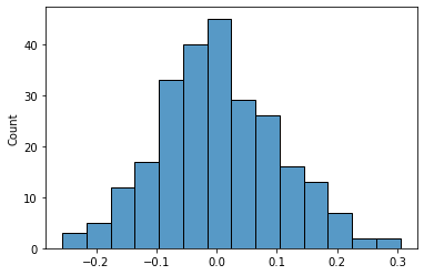
Nosotros can run into that the number of times we had a divergence greater than 0.ii is quite modest. Merely is information technology statistically significant?
diff_g[diff_g>=0.2].shape[0]/diff_g.shape[0] 0.024
Suppose that a significance level of 5% was established before the start of the experiment. In that example, we come across that our event is statistically significant, as the probability of observing a deviation of 12 minutes in the 200 simulations with the re-randomized groups is only 2.4%. If this was due to gamble, information technology would happen only 6 times in 200.
Determination
This commodity covered how conviction intervals and hypothesis tests can be applied to compare differences between samples from two populations. It gives united states a mode to understand if the differences are really statistically significant. We applied the ideas to an experiment that uses simulation and re-randomization to test the departure between a treatment and a control group.
Exercises
You will get the solutions in next calendar week'southward article.
- Physicians hypothesized that the mean time spent in the hospital due to Covid-nineteen before and after the vaccine inverse. A group of 1,000 patients was randomized betwixt a treatment group and a control group. The treatment grouping had already taken the vaccine, while the control group did non. The results show that the treatment grouping's mean time spent in the hospital was 10 days less than the time spent by the command group. The table below summarizes the results for the ane,000 re-randomizations of the data. Based on the information, what is the probability that the treatment group'due south mean is smaller than the ane from the command grouping by 10 days or more? What can you conclude from the experiment's issue (assuming a 5% significance level)?
          diff = [[-17.5,1],
[-15.0, 6],
[-12.five, 15],
[-10.0, 41],
[-7.5, 82],
[-5.0, 43],
[-2.5, 150],
[0., 167],
[2.5, 132],
[five.0, 127],
[vii.5, 173],
[10.0, 38],
[12.five, 18],
[xv.0, vi],
[17.5, 1]]
Answers from concluding week
- Co-ordinate to a large poll from last year, about 85% of houses in Porto have access to high-speed cyberspace. Marco wondered if the proportion had changed and took a random sample of 80 houses and found that 75 had admission to high-speed internet. He wants to use this sample data to test if the proportion actually changed. Assuming that the conditions for inference were met, what would you conclude about the proportion of houses with high-speed internet because a significance level of ane%?
p_0 = 0.85
p = 75/lxxx
n = 80
α = 0.01z = (p-p_0)/np.sqrt(p_0*(1-p_0)/n)
two.191785018798024 p_value = (1-norm.cdf(z))*2 # see that Marco wants to check if the proportion changed, so it is a two-tail examination if p_value < α:
z
print("Reject H0")
else:
impress("Fail to Reject H0") Neglect to Turn down H0
2. Marta owns a fruit store and receives watermelons weekly. The supplier states that they are supposed to counterbalance 1kg. Marta decides to weigh a random sample of 100 watermelons and finds a mean weight of 850g and a standard divergence of 200g. She wants to use this sample data to examination if the mean is smaller than the one claimed by the supplier and renegotiate their contract if this is the example. Assuming that the conditions for inference were met, what should Marta practise (consider a significance level of 5%)?
μ_0 = 1
μ = 0.850
s = 0.two
n = 100
α = 0.05t_star = (μ-μ_0)/(south/np.sqrt(north))
-vii.500000000000001 p_value = t.cdf(t_star, df=n-1) if p_value < α:
t_star
impress("Reject H0")
else:
print("Neglect to Reject H0") Reject H0
Marta should renegotiate the contract with the supplier as the claim that the watermelons weigh 1kg is not truthful for a significance level of 5%.
Source: https://towardsdatascience.com/two-sample-inference-for-the-difference-between-groups-with-python-de91fbee32f9
0 Response to "Review on Difference Between 2 Means Z Distribution"
Post a Comment